Discover and read the best of Twitter Threads about #GoogleSheets
Most recents (24)
¡Atención Seos! ¿Estáis cansados de tener URLs en vuestro sitio web que no generan tráfico? ¡Tenemos la solución! Aquí os dejo una guía paso a paso para eliminar estas URLs sin sufrir consecuencias. ¡Mejoraremos nuestro crawl-budget juntos! #SEO #crawlbudget 👇
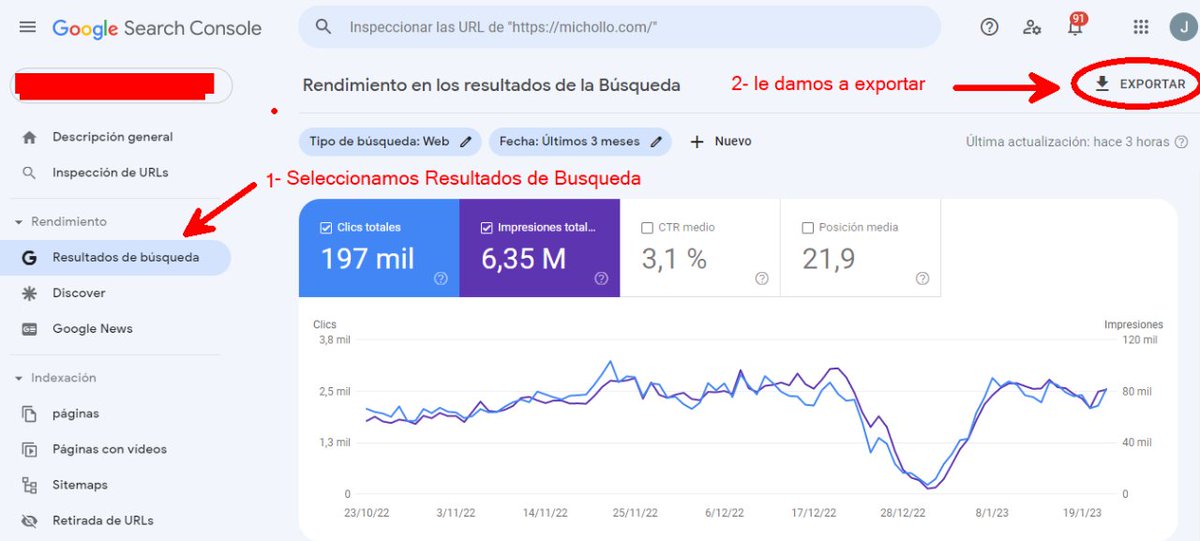
Paso 1: Abrir Google Search Console y acceder a rendimiento o resultados de busqueda. Después, exportar todas las URLs como se muestra en la imagen. #SEO #crawlbudget #GoogleSearchConsole" 

Paso 2: Una vez exportadas las URLs en Google Sheets, seleccionamos la pestaña "Páginas" y filtramos por clic, posición media y CTR (o solo clic si así lo prefieres) #SEO #crawlbudget #GoogleSheets 

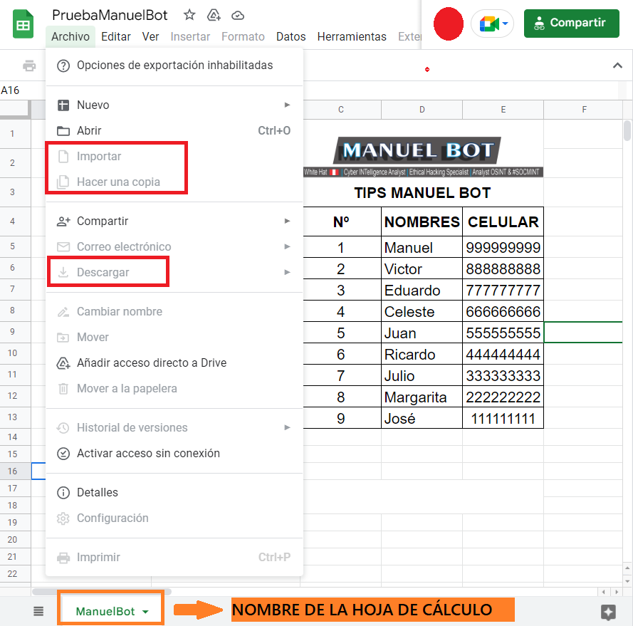
#TipManuelBot: Hola!, les traigo un tip para copiar los datos de un Documento protegido de Google Sheets! (Documento que no se permite hacer copia ni descargar por configuración de acceso al document)
#AnalistaOsint #ToolsOsint #ManuelBot #GoogleSheets #CiberINT
🧵ABRO HILO🧵
#AnalistaOsint #ToolsOsint #ManuelBot #GoogleSheets #CiberINT
🧵ABRO HILO🧵

1⃣ En alguna ocasión habremos accedido a documentos públicos de #GoogleSheet (Hojas de cálculo) y al momento de querer copiar, descargar, importar, imprimir o de hacer una copia del documento, nos topamos con que el document está protegido, pero hay una forma de omitir eso!
⬇️
⬇️

[THREAD]
Comment (bien) compter le nombre de mots dans un texte avec Google Sheets ?
Comment (bien) compter le nombre de mots dans un texte avec Google Sheets ?
Compter le nombre de mots dans un texte est une tâche récurrente en SEO.
Et pourtant, elle n'est pas aussi triviale qu'il n'y paraît.
Je vous montre comment faire avec Google Sheets 👇
Et pourtant, elle n'est pas aussi triviale qu'il n'y paraît.
Je vous montre comment faire avec Google Sheets 👇
1️⃣ Méthode
Il y a plusieurs façons de faire.
Je vais vous en montrer 2 :
- méthode n°1 : compter le nombre d'espaces dans le texte
- méthode n°2 : découper le texte à chaque espace et compter le nombre de valeurs obtenues
Il y a plusieurs façons de faire.
Je vais vous en montrer 2 :
- méthode n°1 : compter le nombre d'espaces dans le texte
- méthode n°2 : découper le texte à chaque espace et compter le nombre de valeurs obtenues
A little step-by-step tutorial to start the week. 👇
Let's create a mini RSS reader in #GoogleSheets to keep us up-to-date with the latest Google Workspace product releases.
We'll be using the IMPORTFEED function to import the Google Workspace Product Updates RSS feed.
Let's create a mini RSS reader in #GoogleSheets to keep us up-to-date with the latest Google Workspace product releases.
We'll be using the IMPORTFEED function to import the Google Workspace Product Updates RSS feed.
First, in cell A1, use the IMPORTFEED function to import the raw RSS feed:
=IMPORTFEED("feeds.feedburner.com/GoogleAppsUpda… ")
=IMPORTFEED("feeds.feedburner.com/GoogleAppsUpda… ")
Then wrap this with the QUERY function to extract the columns we want:
=QUERY(IMPORTFEED("feeds.feedburner.com/GoogleAppsUpda… "),"select Col4, Col1,Col3")
=QUERY(IMPORTFEED("feeds.feedburner.com/GoogleAppsUpda… "),"select Col4, Col1,Col3")
Estaba viendo el directo de @chuisochuisez y ha mencionado el script de @Txtetxu1 que publicó el otro día que puedes ver aquí…
🚨Pues resulta que el otro día me puse y ¡joder! me salió un #appscript que en breve estará en el marketplace de add-on… 👉
🚨Pues resulta que el otro día me puse y ¡joder! me salió un #appscript que en breve estará en el marketplace de add-on… 👉
Soy mú original y lo llame "#GPT3 Tools for #GoogleSheets" Y sí, es #Gratis.
¿Dónde puedes descargarte una copia? Aquí lo tienes: docs.google.com/spreadsheets/d…
¿Cómo funciona?
1. Necesitas cuenta en openai.com/api
2. Haces una copia del libro
3. Extensiones > App Script…
👉
¿Dónde puedes descargarte una copia? Aquí lo tienes: docs.google.com/spreadsheets/d…
¿Cómo funciona?
1. Necesitas cuenta en openai.com/api
2. Haces una copia del libro
3. Extensiones > App Script…
👉
¿Te gusta viajar?🧳
👉 Sabemos que organizar un viaje puede ser retador. Aquí te dejamos 3⃣ herramientas gratuitas de Google para planear tus próximas vacaciones.✈️🌍
Sigue el [HILO]👇
#DíaMundialDelTurismo2022
👉 Sabemos que organizar un viaje puede ser retador. Aquí te dejamos 3⃣ herramientas gratuitas de Google para planear tus próximas vacaciones.✈️🌍
Sigue el [HILO]👇
#DíaMundialDelTurismo2022

1⃣ Descubre atracciones, recorridos y actividades en tu destino con solo un clic.🖱️
👉Con la opción "Qué hacer" de #GoogleViajes puedes encontrar sitios de interés del lugar al que vas y además guardarlos para acceder a ellos desde Google Maps.→ goo.gle/3BOFDxM
👉Con la opción "Qué hacer" de #GoogleViajes puedes encontrar sitios de interés del lugar al que vas y además guardarlos para acceder a ellos desde Google Maps.→ goo.gle/3BOFDxM

2⃣ Lleva la organización de tu viaje a otro nivel con #GoogleSheets📄
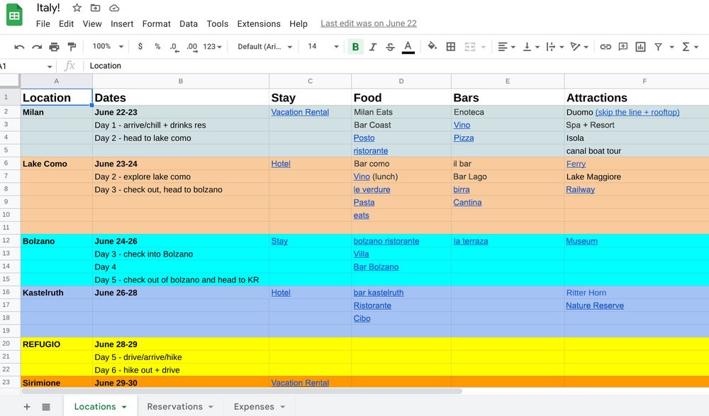
💡Haz un itinerario, junta todas tus reservas o haz una hoja en donde puedas recopilar los gastos que planificaste y los que no.
¿Las has usado antes? 🤔
💡Haz un itinerario, junta todas tus reservas o haz una hoja en donde puedas recopilar los gastos que planificaste y los que no.
¿Las has usado antes? 🤔

🔥 AMAZING SPREADSHEETS 🔥
To some, Google Sheets is just a humble piece of work software...
...but to others, it's a blank canvas to build incredible things with.
10 creations you won't believe are built with #GoogleSheets:
To some, Google Sheets is just a humble piece of work software...
...but to others, it's a blank canvas to build incredible things with.
10 creations you won't believe are built with #GoogleSheets:
1) Wordle in Google Sheets, by @aTylerRobertson
Tyler builds amazing games in Google Sheets, using only the built-in formulas.
His wordle game is just one of many:
👉 zapier.com/blog/wordle-in…
Tyler builds amazing games in Google Sheets, using only the built-in formulas.
His wordle game is just one of many:
👉 zapier.com/blog/wordle-in…

2) Minesweeper in Google Sheets, by @KieransSheets
This is a beautifully constructed game that uses Apps Script (Google Sheets code) to recreate the classic minesweeper actions.
Kieran has documented the build in amazing detail too!
👉 kierandixon.com/google-sheets-…
This is a beautifully constructed game that uses Apps Script (Google Sheets code) to recreate the classic minesweeper actions.
Kieran has documented the build in amazing detail too!
👉 kierandixon.com/google-sheets-…

Document Studio helps you automate work with the help of Google Sheets and Google Forms.
workspace.google.com/marketplace/ap…
workspace.google.com/marketplace/ap…
The first version of Document Studio launched in 2017 and we've since added tons of new features and integrations. It took us more than 18 months of coding+testing to get here.
digitalinspiration.com/docs/document-…
digitalinspiration.com/docs/document-…

The SEQUENCE function is an amazingly useful function in #GoogleSheets. It lets you create sequences of numbers from a single formula. The obvious use case is to create a count up 1, 2, 3, 4, 5 etc.
But did you know you can easily create a count down in your Sheets too? 👇
But did you know you can easily create a count down in your Sheets too? 👇
This single, simple formula:
=SEQUENCE(100,1,100,-1)
counts down from 100 e.g. 100, 99, 98, 97, 96...1
To count down from some other number, for example 50, change it as follows:
=SEQUENCE(50,1,50,-1)
Easy-peasy!
=SEQUENCE(100,1,100,-1)
counts down from 100 e.g. 100, 99, 98, 97, 96...1
To count down from some other number, for example 50, change it as follows:
=SEQUENCE(50,1,50,-1)
Easy-peasy!
The four numbers you enter as arguments to the SEQUENCE function represent:
✅ Number of rows (e.g. 100)
✅ Number of columns (e.g. 1)
✅ Start number (e.g. 100)
✅ Step to increase/decrease by (e.g. -1)
Arguments 2, 3 and 4 are also optional.
✅ Number of rows (e.g. 100)
✅ Number of columns (e.g. 1)
✅ Start number (e.g. 100)
✅ Step to increase/decrease by (e.g. -1)
Arguments 2, 3 and 4 are also optional.
If you create #GoogleSheets that multiple people use, one super helpful thing you can do is add a sidebar to your Sheets, containing key info or instructions.
Today I'm going to show you how to create sidebars using the group columns feature...
Today I'm going to show you how to create sidebars using the group columns feature...
STEP 1️⃣
Highlight some columns, right click, and choose Group columns.
This adds a button above the columns, which you can toggle to show/hide these grouped columns.
Highlight some columns, right click, and choose Group columns.
This adds a button above the columns, which you can toggle to show/hide these grouped columns.
STEP 2️⃣
Right-click on the +/- button and select left or right to set the +/- toggle button to be on the left or right of the group.
Right-click on the +/- button and select left or right to set the +/- toggle button to be on the left or right of the group.
In today's #GoogleSheets tip, I'm going to show you how to highlight the top 5 values in your data.
There are loads of ways to do this, like adding a filter and sorting the values highest to lowest, but today we're going to be using formulas and conditional formatting.
There are loads of ways to do this, like adding a filter and sorting the values highest to lowest, but today we're going to be using formulas and conditional formatting.
Here's the dataset we'll be using. Let's dive in!
1️⃣ Highlight your data, but exclude the header row, i.e. A2:C21 in this example
2️⃣ Open the menu: Format > Conditional formatting
3️⃣ Under Format rules, select Custom formula is
1️⃣ Highlight your data, but exclude the header row, i.e. A2:C21 in this example
2️⃣ Open the menu: Format > Conditional formatting
3️⃣ Under Format rules, select Custom formula is

4️⃣ Add one of the following formulas:
=$C2>=LARGE($C$2:$C$21,5)
or
=RANK($C2,$C$2:$C$21)<=5
The functions LARGE and RANK can all identify the position of a value relative to others around it.
5️⃣ Choose your format options, e.g. highlight the rows yellow.
=$C2>=LARGE($C$2:$C$21,5)
or
=RANK($C2,$C$2:$C$21)<=5
The functions LARGE and RANK can all identify the position of a value relative to others around it.
5️⃣ Choose your format options, e.g. highlight the rows yellow.
Today I want to show you a quick way to add an ID column to your #GoogleSheets tables, using the SEQUENCE and COUNTA functions.
It's a quick way to see how many records you have in your table.
Let's go! 👇
(1/9)
It's a quick way to see how many records you have in your table.
Let's go! 👇
(1/9)
Did you know you can publish your #GoogleSheets as web pages?
You can then share these web pages with the world, so people can see your Sheet as a distinct, lightweight webpage.
It's a good idea if you want to show the Sheet to a very large audience.
(1/3)
You can then share these web pages with the world, so people can see your Sheet as a distinct, lightweight webpage.
It's a good idea if you want to show the Sheet to a very large audience.
(1/3)
The QUERY function in #GoogleSheets is pretty much the most powerful function in the spreadsheet world.
It operates on your data and has the functionality of many other functions, like sorting, aggregation, filtering, etc.
It's like a pivot table in function form.
(1/4)
It operates on your data and has the functionality of many other functions, like sorting, aggregation, filtering, etc.
It's like a pivot table in function form.
(1/4)
It's a tricky function to learn because it's so different from regular functions. You use query language to write a statement that operates on your data.
Here's an example:
=QUERY(A1:E100,"select B, D, E where D = 'Europe'",1)
(2/4)
Here's an example:
=QUERY(A1:E100,"select B, D, E where D = 'Europe'",1)
(2/4)
Automate your #GoogleAds budget pacing for FREE.
To get started, you’ll need:
🖥️ Your #GoogleAds account
📄 #GoogleSheets
➕ The #GoogleAds Add-on for #GoogleSheets
💸 Campaign budgets
📅 Campaign end dates
Here’s what you need to do...🧵👇
To get started, you’ll need:
🖥️ Your #GoogleAds account
📄 #GoogleSheets
➕ The #GoogleAds Add-on for #GoogleSheets
💸 Campaign budgets
📅 Campaign end dates
Here’s what you need to do...🧵👇
Using the Google Ads Add-on, create a report that pulls cost data per campaign, per account, for the current month.
Set it to automatically refresh daily.
Set it to automatically refresh daily.
Columns you need from the Add-on report:
- Customer ID
- Account
- Campaign
- Campaign ID
- Cost.
You'll need to manually add new columns at the end:
- Budget
- Budget Type
- Today’s Date
- End Date
- Total Campaign Budget
- Action
- Customer ID
- Account
- Campaign
- Campaign ID
- Cost.
You'll need to manually add new columns at the end:
- Budget
- Budget Type
- Today’s Date
- End Date
- Total Campaign Budget
- Action
I've updated the #tether attestation #googlesheets analysis. A few changes including fixing a glaring error 😳 #commercialpaper analysis h/t to @accountantInc catching the mistake. Document consolidates all reported quarters to date >>> bit.ly/3Kzkjz2 

The #tether #commercialpaper section has been expanded/updated to show not just the net changes but the new issues/rollovers etc.... 

The purpose of the #commercialpaper analysis was to highlight that the reported $6.4B reduction in CP was only half the story....and it kinda shits me that the numbers are just trumpeted by most news as is... 

Have been working through $CEL #celsiusnetwork's $750m Series B round. Will share #googlesheets file tomorrow. Here's a preview.
3 Dec 2021 #Celsius resolved to issue up-to 36,930 Series B shares at a price of US$20,469 per share. As at 2 Feb 2022 total of 32,182 Series B shares had been issued. I'm presuming #bnktothefuture will have closed out the balance. 

The #Celsius Cap table (as at 2 Feb) with pre/post money for each issue. 

#CryptoEducation Gems [Mega Thread]
A navigational aid for the variety of projects featured in current @gitcoin #GR13:
A curated list of projects that are helping blockchains become an integral part of the world by empowering people with knowledge and education. 🤓🔖💪
1/N
A navigational aid for the variety of projects featured in current @gitcoin #GR13:
A curated list of projects that are helping blockchains become an integral part of the world by empowering people with knowledge and education. 🤓🔖💪
1/N
🔎 @LearnWeb3DAO / @haardikkk
(education system)
For open-minded individuals, interested in everything they need to know in order to become a #Web3 native.
A very rich resource with a fast-growing userbase of Web3 students.
👉gitcoin.co/grants/5066/le…
2/N #GR13
(education system)
For open-minded individuals, interested in everything they need to know in order to become a #Web3 native.
A very rich resource with a fast-growing userbase of Web3 students.
👉gitcoin.co/grants/5066/le…
2/N #GR13
🔎 Odyssey DAO / @odyssey_dao
(Educational DAO / resource)
For #Web3 newcomers interested in high-quality learning material with a variety of learning paths.
👉gitcoin.co/grants/5016/od…
3/N #GR13
(Educational DAO / resource)
For #Web3 newcomers interested in high-quality learning material with a variety of learning paths.
👉gitcoin.co/grants/5016/od…
3/N #GR13
Let's learn how to use custom checkbox values to use checkboxes directly in #GoogleSheets formulas. 🎉
(1/6)
(1/6)
Usá la búsqueda avanzada de @gmail para borrar archivos pesados que ya no necesites. 📪
🔎 En el cuadro de búsqueda, tipeá "has:attachment larger:10M". Si es necesario, podés sustituir el 10 por un número de peso más grande. 😎
🔎 En el cuadro de búsqueda, tipeá "has:attachment larger:10M". Si es necesario, podés sustituir el 10 por un número de peso más grande. 😎
En @YouTube podés compartir un momento específico de un video, siguiendo estos pasos:
👉 Desplazate hasta el momento que desees.
👉 Clic derecho y pulsá en "Copiar la URL del video a partir del minuto actual".
👉 Quien abra el link verá el video a partir de ese momento.
👉 Desplazate hasta el momento que desees.
👉 Clic derecho y pulsá en "Copiar la URL del video a partir del minuto actual".
👉 Quien abra el link verá el video a partir de ese momento.
💜 Turn your GoogleSheets into a web scraping machine for SEO 💜
There is a lot that you can accomplish w/ GSheets. Let's start the new year with some super cool productivity hacks w/ the IMPORTXML function of it💡
#WebScraping #ProductivityHacks #GoogleSheets #SEO
It's a 🧵
There is a lot that you can accomplish w/ GSheets. Let's start the new year with some super cool productivity hacks w/ the IMPORTXML function of it💡
#WebScraping #ProductivityHacks #GoogleSheets #SEO
It's a 🧵
A great way to be more efficient in #GoogleSheets is to learn basic shortcuts for selecting data.
That's what I'm going to show you today - how to select data for formulas without your hands leaving the keyboard. ⌨️
It's so much quicker than grabbing the mouse! 🖱️
That's what I'm going to show you today - how to select data for formulas without your hands leaving the keyboard. ⌨️
It's so much quicker than grabbing the mouse! 🖱️
I remember how awkward it felt when I first learned these shortcuts, and how it was initially slower than just using the mouse to highlight the data.
But after a few days, it was significantly quicker than using the mouse. And it will be for you too.
Here we go ⬇️
But after a few days, it was significantly quicker than using the mouse. And it will be for you too.
Here we go ⬇️
1️⃣
Move quickly to the last non-blank cell in a row or column:
PC/Chromebook: Ctrl + ⬆⬇⬅➡
Mac: ⌘ + ⬆⬇⬅➡
Move quickly to the last non-blank cell in a row or column:
PC/Chromebook: Ctrl + ⬆⬇⬅➡
Mac: ⌘ + ⬆⬇⬅➡
The OFFSET function is not a function you need particularly often, but it's worth knowing about because it allows you to move ranges around very easily.
#GoogleSheets thread. Let's go. 👇
#GoogleSheets thread. Let's go. 👇
The OFFSET function returns a reference to a range that is offset from a starting point in a worksheet.
For example, in the table shown in this image, imagine you want to align these columns at the top of the column.
For example, in the table shown in this image, imagine you want to align these columns at the top of the column.

The OFFSET function can do this with a single formula for each column, which is quicker and easier than copy-pasting or creating complex nested formulas.
The OFFSET formula in this example is:
=offset( B2:B6, 1, 0, count(B2:B6) )
The OFFSET formula in this example is:
=offset( B2:B6, 1, 0, count(B2:B6) )
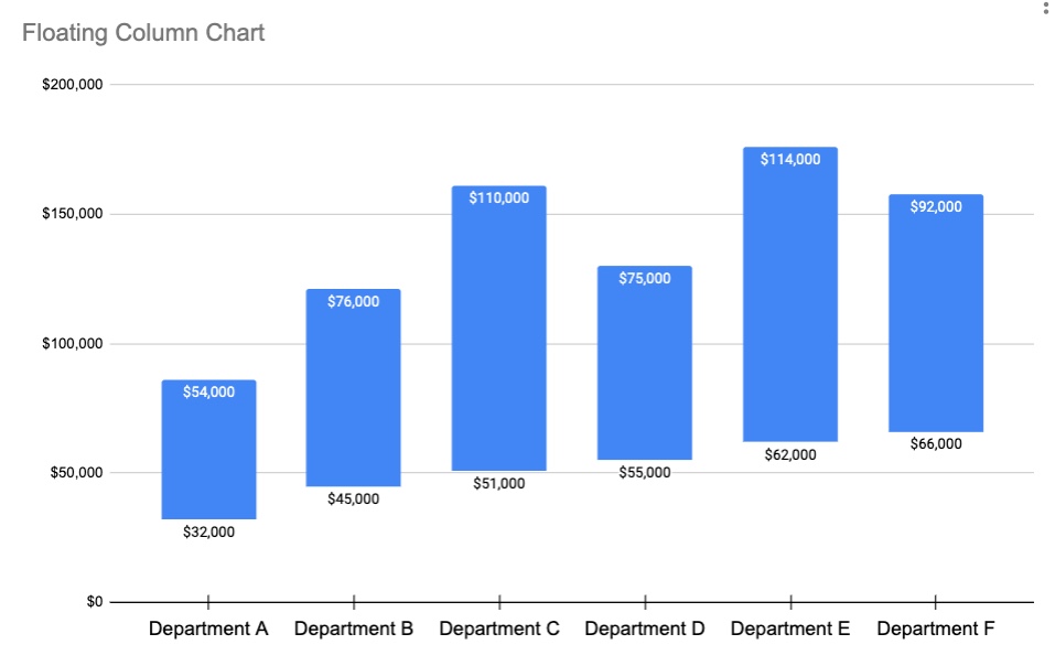
Have you come across floating bar (or column) charts before?
They're a useful way to show data when you want to compare ranges or high and low values.
For example, you can use floating bar charts with salary data, weather data, stock prices, blood pressure readings, etc.
They're a useful way to show data when you want to compare ranges or high and low values.
For example, you can use floating bar charts with salary data, weather data, stock prices, blood pressure readings, etc.

To create a floating bar (or column) chart in #GoogleSheets, you’ll need two series in your dataset, e.g. a set of low values and a set of high values, like this salary range dataset. 

Then follow these steps...
1. Highlight the data and Insert > Chart
2. In Setup, choose a Bar Chart (horizontal) or Column Chart (vertical)
3. Still in the chart setup menu, set the Stacking to be “Standard”
4. Go to the Customize menu
(continued in next tweet)
1. Highlight the data and Insert > Chart
2. In Setup, choose a Bar Chart (horizontal) or Column Chart (vertical)
3. Still in the chart setup menu, set the Stacking to be “Standard”
4. Go to the Customize menu
(continued in next tweet)


